2 Statistical Learning

Conceptual

Question 1

(a) Better: flexible method incorporates the data better when the sample size is large enough.

(b) Worse: The data set leads to the ‘Curse of Dimensionality’, flexible model will tend to be more overfitting, meaning it will try to follow the error (noise) too closely.

(c) Better: Flexible methods perform better on non-linear datasets as they have more degrees of freedom to approximate a non-linear.

(d) Worse: A flexible model would likely overfit, due to more closely fitting the noise in the error terms than an inflexible method. In other words, the data points will be far from f (ideal function to describe the data) if the variance of the error terms is very high. This hints that that f is linear and so a simpler model would be better to be able to estimate f.

Question 2

(a) Regression Problem: Since it is a quantitative problem
Inference: We are interested in the factors which affect CEO salary
n = 500
p = 3 (Profit, number of employees, industry)

(b) Classification Problem: Since it is binary (success or failure)
Prediction: We are interested in the success or failure of the product
n = 20
p = 13 (Price charged, marketing budget, competition price + 10 other)

(c) Regression Problem
Prediction: We are interested in the % change in the USD/Euro exchange rate
n = 52
p = 3 (% change in the US market, % change in the British market, % change in the German market)

Question 3

(a) AI-generated

(b) Squared Bias: Decreases with more flexibility (generally more flexible methods results in less bias)

Variance: Increases with more flexibility

Training Error: Continues to reduce as flexibility grows, meaning the model is too close to the training data.

Test Error: Decreases initially, and reaches the optimal point where it gets flat, then it starts to increase again, meaning an overfitted data

Bayes (irreducible) Error: Flat/Fixed, since it can’t be reduced any more

Question 4

(a) Three real-life applications in which classification might be useful

1. Email Spam Detection

Response: Spam(1) or Not Spam(0)
Predictors: some special words, special links, other
Goal: Prediction — we care more about classifying new emails correctly than about interpreting which word exactly causes spam.

2. Loan Default Risk

Respone: Default(1) or Won’t Default(0)
Predictors: income, credit score, education, etc
Goal: Prediction/Inference — banks want to predict default risk, but also understand which factors matter most

3. Stock Price

Response: Stock increases(1) or Stock goes down(0)
Predictors: Financial Statements, Ratio Analysis, Competitors price, etc
Goal: Prediction — we are interested in making the future movements of the stock price.

(b) Three real-life applications in which regression might be useful:

1. House Price Estimation

Response: House price (in $).
Predictors: square footage, number of bedrooms, location, age of house.
Goal: Prediction — estimate the price of houses not yet sold.

2. Salary Determination

Response: Employee salary (in $).
Predictors: years of experience, education level, industry, job role.
Goal: Inference — HR might want to know which factors (experience vs. education) most strongly drive salaries.

3. Insurance Premium Calculation

Response: Annual premium amount.
Predictors: age, medical history, smoking status, BMI.
Goal: Both — insurers need prediction for pricing policies, but also inference to understand key risk drivers.

(c) Three real-life applications in which cluster analysis might be useful:

1. Customer Segmentation in Retail

Predictors: purchase history, shopping frequency, spending amounts.
Goal: Identify customer groups (e.g., bargain-hunters vs. high spenders) for targeted marketing.

2. Genetic Research

Predictors: gene expression levels.
Goal: Cluster similar genes/patients to identify subtypes of diseases.

3. Social Media Communities

Predictors: interaction patterns, hashtags used, follower networks.
Goal: Find natural clusters of users (e.g., sports fans, political groups, hobby communities).

Question 5

Advantages of a More Flexible Approach

Better fit to complex patterns: Can capture nonlinear relationships and intricate interactions between variables.
Lower bias: Since fewer assumptions are made about the functional form, the model can adapt closely to the data.
High predictive power: Often yields better test accuracy if enough data is available.

Disadvantages of a More Flexible Approach

Risk of overfitting: May capture noise in the training data instead of the true signal.
Higher variance: Predictions can change drastically with new data.
Interpretability: Flexible models are often “black boxes” (e.g., random forests, neural nets).
Computational cost: More data and resources needed for training.

Advantages of a Less Flexible Approach

Simplicity: Easy to implement, interpret, and explain to stakeholders.
Low variance: Less sensitive to small changes in the dataset.
Efficient: Works well with smaller datasets, requires less computation.
Inference: Easier to test hypotheses and understand relationships between predictors and response.

Disadvantages of a Less Flexible Approach

High bias: May oversimplify reality by assuming linearity or ignoring interactions.
Poor fit for complex relationships: If the true relationship is nonlinear, performance suffers.

When to prefer More Flexible Approaches

When prediction accuracy is the main goal.
When the relationship between predictors and response is complex and nonlinear.
When you have large amounts of data to reduce variance and prevent overfitting.

When to prefer Less Flexible Approaches

When the primary goal is inference/interpretability (understanding which predictors matter).
When you have limited data, flexible models overfit easily with small datasets.
When stakeholders (like regulators, executives) need transparent models.

Question 6

Parametric: Assume a functional form (e.g., linear regression), then estimate a few parameters.

Advantage: Works with small data, simple, interpretable, fast.
Disadvantage: Risk of bias if model form is wrong, limited flexibility.

Non-Parametric: No strict form, model is shaped by the data (e.g., KNN, trees).

Advantage: Very flexible, can capture complex patterns.
Disadvantage: Needs lots of data, higher variance, less interpretable, slower.

Question 7

(a) Computing the Euclidean distance between each observation and the test point, X1 = X2 = X3 = 0

(data.set <- data.frame(
  "X1" = c(0,2,0,0,-1,1),
  "X2" = c(3,0,1,1,0,1),
  "X3" = c(0,0,3,2,1,1),
  "Y" = c("Red","Red","Red","Green","Green","Red")
  ))   # A given data set

  X1 X2 X3     Y
1  0  3  0   Red
2  2  0  0   Red
3  0  1  3   Red
4  0  1  2 Green
5 -1  0  1 Green
6  1  1  1   Red

euclidian.distance <- 
  function(X, pred.data){
    # 'X' here represents a vector of points
    distance = sqrt((X[1]-pred.data[1])^2 +
                      (X[2]-pred.data[2])^2 +
                      (X[3]-pred.data[3])^2) 
    return(distance)
  }  # A function to compute euclidian distance

X <- data.set[,-4]    # Taking only the given X co-ordinates
Prediction.coordinates <- c(0,0,0) # Prediction co-ordinates

distance <- numeric()
for(i in 1:nrow(X)){
  distance[i] = as.matrix(euclidian.distance(X[i,], Prediction.coordinates))
}

distance <- as.matrix(distance)

cat("\n",
  "dist(New,Obs1) =",distance[1,1],"\n",
  "dist(New,Obs2) =",distance[2,1],"\n",
  "dist(New,Obs3) =",distance[3,1],"\n",
  "dist(New,Obs4) =",distance[4,1],"\n",
  "dist(New,Obs5) =",distance[5,1],"\n",
  "dist(New,Obs6) =",distance[6,1],"\n"
  )


 dist(New,Obs1) = 3 
 dist(New,Obs2) = 2 
 dist(New,Obs3) = 3.162278 
 dist(New,Obs4) = 2.236068 
 dist(New,Obs5) = 1.414214 
 dist(New,Obs6) = 1.732051

(b)

(Y <- data.set[,4]) # All possible given ouputs

[1] "Red"   "Red"   "Red"   "Green" "Green" "Red"

KNN <- 
  function(K){
    Y[which.min(abs(distance[,1]-K))]
  }

cat("K-Nearest Neighbour for K = 1 predicts it to be",KNN(1))

K-Nearest Neighbour for K = 1 predicts it to be Green

(c)

cat("K-Nearest Neighbour for K = 3 predicts it to be",KNN(3))

K-Nearest Neighbour for K = 3 predicts it to be Red

APPLIED

Question 8

Running the ‘ISLR2’ package

# install.packages("ISLR2")
library(ISLR2)

(a)

college <- College # naming as per question

(b)

# View(college) #
head(college)

                             Private Apps Accept Enroll Top10perc Top25perc
Abilene Christian University     Yes 1660   1232    721        23        52
Adelphi University               Yes 2186   1924    512        16        29
Adrian College                   Yes 1428   1097    336        22        50
Agnes Scott College              Yes  417    349    137        60        89
Alaska Pacific University        Yes  193    146     55        16        44
Albertson College                Yes  587    479    158        38        62
                             F.Undergrad P.Undergrad Outstate Room.Board Books
Abilene Christian University        2885         537     7440       3300   450
Adelphi University                  2683        1227    12280       6450   750
Adrian College                      1036          99    11250       3750   400
Agnes Scott College                  510          63    12960       5450   450
Alaska Pacific University            249         869     7560       4120   800
Albertson College                    678          41    13500       3335   500
                             Personal PhD Terminal S.F.Ratio perc.alumni Expend
Abilene Christian University     2200  70       78      18.1          12   7041
Adelphi University               1500  29       30      12.2          16  10527
Adrian College                   1165  53       66      12.9          30   8735
Agnes Scott College               875  92       97       7.7          37  19016
Alaska Pacific University        1500  76       72      11.9           2  10922
Albertson College                 675  67       73       9.4          11   9727
                             Grad.Rate
Abilene Christian University        60
Adelphi University                  56
Adrian College                      54
Agnes Scott College                 59
Alaska Pacific University           15
Albertson College                   55

(c)

# i.
summary(college)

 Private        Apps           Accept          Enroll       Top10perc    
 No :212   Min.   :   81   Min.   :   72   Min.   :  35   Min.   : 1.00  
 Yes:565   1st Qu.:  776   1st Qu.:  604   1st Qu.: 242   1st Qu.:15.00  
           Median : 1558   Median : 1110   Median : 434   Median :23.00  
           Mean   : 3002   Mean   : 2019   Mean   : 780   Mean   :27.56  
           3rd Qu.: 3624   3rd Qu.: 2424   3rd Qu.: 902   3rd Qu.:35.00  
           Max.   :48094   Max.   :26330   Max.   :6392   Max.   :96.00  
   Top25perc      F.Undergrad     P.Undergrad         Outstate    
 Min.   :  9.0   Min.   :  139   Min.   :    1.0   Min.   : 2340  
 1st Qu.: 41.0   1st Qu.:  992   1st Qu.:   95.0   1st Qu.: 7320  
 Median : 54.0   Median : 1707   Median :  353.0   Median : 9990  
 Mean   : 55.8   Mean   : 3700   Mean   :  855.3   Mean   :10441  
 3rd Qu.: 69.0   3rd Qu.: 4005   3rd Qu.:  967.0   3rd Qu.:12925  
 Max.   :100.0   Max.   :31643   Max.   :21836.0   Max.   :21700  
   Room.Board       Books           Personal         PhD        
 Min.   :1780   Min.   :  96.0   Min.   : 250   Min.   :  8.00  
 1st Qu.:3597   1st Qu.: 470.0   1st Qu.: 850   1st Qu.: 62.00  
 Median :4200   Median : 500.0   Median :1200   Median : 75.00  
 Mean   :4358   Mean   : 549.4   Mean   :1341   Mean   : 72.66  
 3rd Qu.:5050   3rd Qu.: 600.0   3rd Qu.:1700   3rd Qu.: 85.00  
 Max.   :8124   Max.   :2340.0   Max.   :6800   Max.   :103.00  
    Terminal       S.F.Ratio      perc.alumni        Expend     
 Min.   : 24.0   Min.   : 2.50   Min.   : 0.00   Min.   : 3186  
 1st Qu.: 71.0   1st Qu.:11.50   1st Qu.:13.00   1st Qu.: 6751  
 Median : 82.0   Median :13.60   Median :21.00   Median : 8377  
 Mean   : 79.7   Mean   :14.09   Mean   :22.74   Mean   : 9660  
 3rd Qu.: 92.0   3rd Qu.:16.50   3rd Qu.:31.00   3rd Qu.:10830  
 Max.   :100.0   Max.   :39.80   Max.   :64.00   Max.   :56233  
   Grad.Rate     
 Min.   : 10.00  
 1st Qu.: 53.00  
 Median : 65.00  
 Mean   : 65.46  
 3rd Qu.: 78.00  
 Max.   :118.00

# ii.
pairs(college[,1:10], cex = 0.1)

# iii.
boxplot(Outstate ~ Private, data = college)

# iv.
college$Elite <- as.factor(ifelse(college$Top10perc > 50, "Yes", "No"))

summary(college$Elite)

 No Yes 
699  78

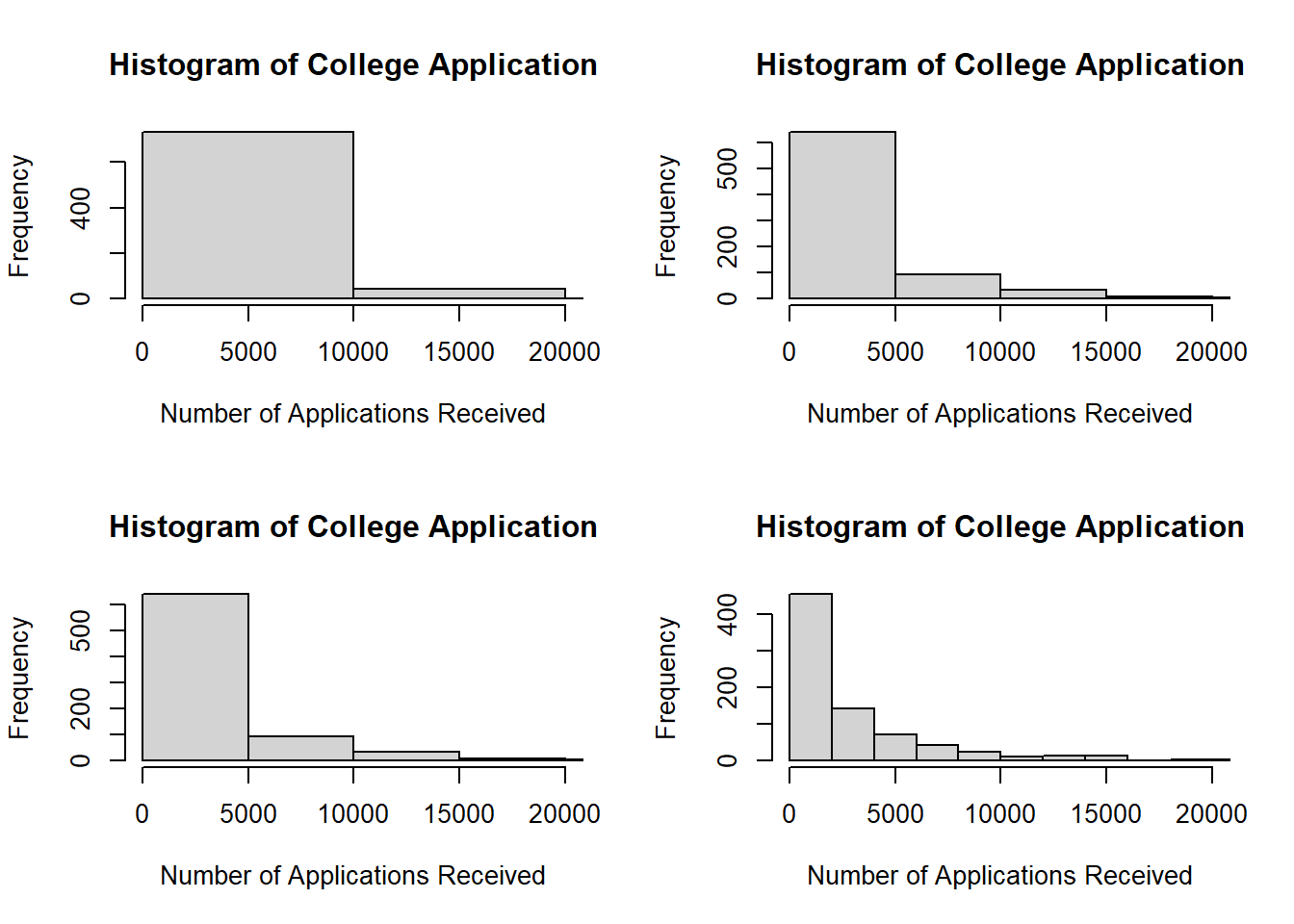
# v.
par(mfrow = c(2,2))

# FOR COLLEGE APPLICATIONS RECEIVED
for(n in c(5,10,15,20)){
  hist(college$Apps, 
       xlab = "Number of Applications Received",
       main = "Histogram of College Application",
       breaks = n,
       xlim = c(0,20000))
}

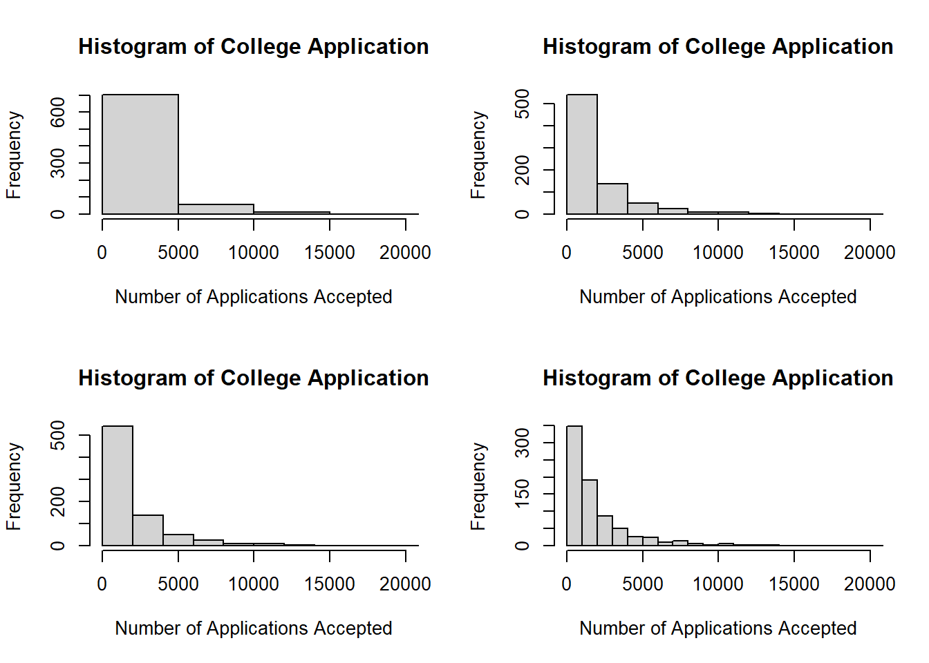
par(mfrow = c(2,2))

# FOR COLLEGE APPLICATIONS ACCEPTED
for(n in c(5,10,15,20)){
  hist(college$Accept, 
       xlab = "Number of Applications Accepted",
       main = "Histogram of College Application",
       breaks = n,
       xlim = c(0,20000))
}

par(mfrow = c(1,1))

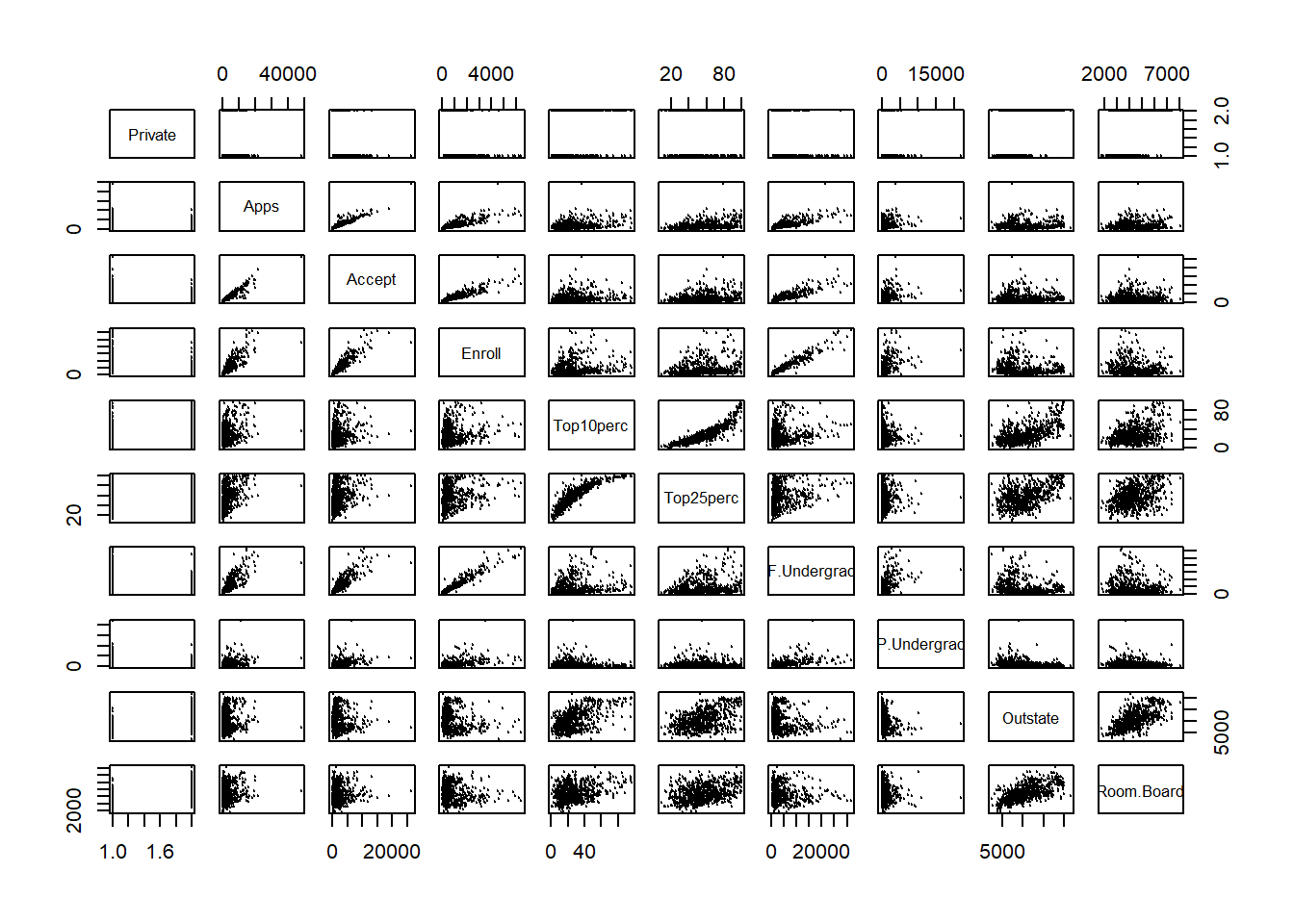
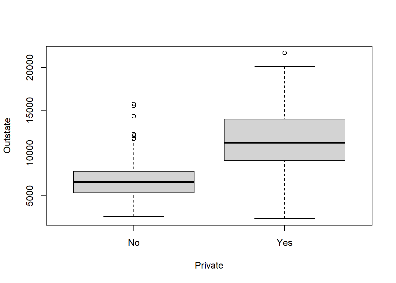
# vi.
# Making a linear model with all variables
Model1 <- lm(Accept~.,data=College)
summary(Model1)


Call:
lm(formula = Accept ~ ., data = College)

Residuals:
    Min      1Q  Median      3Q     Max 
-3628.2  -186.3     5.1   197.0  3476.0 

Coefficients:
              Estimate Std. Error t value Pr(>|t|)    
(Intercept) -2.896e+02  2.101e+02  -1.378  0.16850    
PrivateYes   1.654e+02  7.128e+01   2.320  0.02058 *  
Apps         4.201e-01  1.079e-02  38.924  < 2e-16 ***
Enroll       1.162e+00  8.749e-02  13.276  < 2e-16 ***
Top10perc   -2.765e+01  2.847e+00  -9.713  < 2e-16 ***
Top25perc    9.246e+00  2.296e+00   4.026 6.24e-05 ***
F.Undergrad -1.870e-02  1.686e-02  -1.109  0.26773    
P.Undergrad -3.368e-02  1.652e-02  -2.039  0.04183 *  
Outstate     6.090e-02  9.690e-03   6.286 5.51e-10 ***
Room.Board  -1.196e-02  2.501e-02  -0.478  0.63272    
Books        1.580e-02  1.227e-01   0.129  0.89756    
Personal    -4.552e-02  3.243e-02  -1.404  0.16080    
PhD          4.680e+00  2.387e+00   1.961  0.05025 .  
Terminal     6.402e-01  2.623e+00   0.244  0.80724    
S.F.Ratio   -4.666e+00  6.699e+00  -0.697  0.48627    
perc.alumni -5.529e+00  2.102e+00  -2.630  0.00871 ** 
Expend      -2.952e-02  6.432e-03  -4.590 5.19e-06 ***
Grad.Rate   -1.231e+00  1.526e+00  -0.807  0.42000    
---
Signif. codes:  0 '***' 0.001 '**' 0.01 '*' 0.05 '.' 0.1 ' ' 1

Residual standard error: 536 on 759 degrees of freedom
Multiple R-squared:  0.9532,    Adjusted R-squared:  0.9522 
F-statistic: 909.9 on 17 and 759 DF,  p-value: < 2.2e-16

# Using this model to determine all the significant parameters which comes out 
# to be:
# -> Private
# -> Apps
# -> Enroll
# -> Top10perc
# -> Top25perc
# -> P.Undergrad
# -> Outstate
# -> perc.alumni
# -> Expend
# Making another model with these parameters only:

Model2 <- lm(Accept ~ Private + Apps + Enroll + Top10perc + Top25perc +
               P.Undergrad + Outstate + perc.alumni + Expend,
             data=College)
summary(Model2)


Call:
lm(formula = Accept ~ Private + Apps + Enroll + Top10perc + Top25perc + 
    P.Undergrad + Outstate + perc.alumni + Expend, data = College)

Residuals:
    Min      1Q  Median      3Q     Max 
-3728.9  -187.9    -2.3   212.3  3550.0 

Coefficients:
              Estimate Std. Error t value Pr(>|t|)    
(Intercept) -2.761e+02  9.134e+01  -3.023  0.00258 ** 
PrivateYes   1.120e+02  6.557e+01   1.709  0.08788 .  
Apps         4.168e-01  1.047e-02  39.810  < 2e-16 ***
Enroll       1.085e+00  4.534e-02  23.933  < 2e-16 ***
Top10perc   -2.740e+01  2.824e+00  -9.700  < 2e-16 ***
Top25perc    1.005e+01  2.242e+00   4.483 8.49e-06 ***
P.Undergrad -3.612e-02  1.552e-02  -2.327  0.02020 *  
Outstate     6.801e-02  8.312e-03   8.182 1.16e-15 ***
perc.alumni -4.846e+00  2.015e+00  -2.405  0.01639 *  
Expend      -2.678e-02  5.882e-03  -4.552 6.16e-06 ***
---
Signif. codes:  0 '***' 0.001 '**' 0.01 '*' 0.05 '.' 0.1 ' ' 1

Residual standard error: 538 on 767 degrees of freedom
Multiple R-squared:  0.9524,    Adjusted R-squared:  0.9518 
F-statistic:  1705 on 9 and 767 DF,  p-value: < 2.2e-16

# Adjusted R-squared dropped but only by 0.0004, that doesn't make Model1 any
# better than Model2 with so much less parameters.

AIC(Model1)

[1] 11990.35

AIC(Model2)

[1] 11988.27

# AIC dropped

# Another Model with even less parameters
Model3 <- update(Model2, .~. -Private - P.Undergrad - perc.alumni)
summary(Model3)


Call:
lm(formula = Accept ~ Apps + Enroll + Top10perc + Top25perc + 
    Outstate + Expend, data = College)

Residuals:
    Min      1Q  Median      3Q     Max 
-3758.7  -180.9    -3.7   206.5  3618.8 

Coefficients:
              Estimate Std. Error t value Pr(>|t|)    
(Intercept) -2.766e+02  8.696e+01  -3.180  0.00153 ** 
Apps         4.186e-01  1.039e-02  40.308  < 2e-16 ***
Enroll       1.034e+00  4.266e-02  24.240  < 2e-16 ***
Top10perc   -2.695e+01  2.816e+00  -9.569  < 2e-16 ***
Top25perc    9.260e+00  2.245e+00   4.125 4.12e-05 ***
Outstate     7.040e-02  7.129e-03   9.875  < 2e-16 ***
Expend      -2.865e-02  5.896e-03  -4.859 1.43e-06 ***
---
Signif. codes:  0 '***' 0.001 '**' 0.01 '*' 0.05 '.' 0.1 ' ' 1

Residual standard error: 541.7 on 770 degrees of freedom
Multiple R-squared:  0.9515,    Adjusted R-squared:  0.9512 
F-statistic:  2520 on 6 and 770 DF,  p-value: < 2.2e-16

AIC(Model3)

[1] 11995.87

# AIC increased by ~2 points

anova(Model2, Model3)

Analysis of Variance Table

Model 1: Accept ~ Private + Apps + Enroll + Top10perc + Top25perc + P.Undergrad + 
    Outstate + perc.alumni + Expend
Model 2: Accept ~ Apps + Enroll + Top10perc + Top25perc + Outstate + Expend
  Res.Df       RSS Df Sum of Sq     F   Pr(>F)   
1    767 221996912                               
2    770 225916474 -3  -3919562 4.514 0.003789 **
---
Signif. codes:  0 '***' 0.001 '**' 0.01 '*' 0.05 '.' 0.1 ' ' 1

# Another Model
Model4 <- update(Model2, .~. -Private)
summary(Model4)


Call:
lm(formula = Accept ~ Apps + Enroll + Top10perc + Top25perc + 
    P.Undergrad + Outstate + perc.alumni + Expend, data = College)

Residuals:
    Min      1Q  Median      3Q     Max 
-3714.3  -189.2     0.3   213.5  3601.4 

Coefficients:
              Estimate Std. Error t value Pr(>|t|)    
(Intercept) -2.315e+02  8.762e+01  -2.642  0.00842 ** 
Apps         4.152e-01  1.044e-02  39.763  < 2e-16 ***
Enroll       1.068e+00  4.434e-02  24.098  < 2e-16 ***
Top10perc   -2.725e+01  2.827e+00  -9.642  < 2e-16 ***
Top25perc    9.827e+00  2.241e+00   4.385 1.32e-05 ***
P.Undergrad -3.952e-02  1.541e-02  -2.565  0.01050 *  
Outstate     7.404e-02  7.534e-03   9.828  < 2e-16 ***
perc.alumni -4.540e+00  2.009e+00  -2.259  0.02415 *  
Expend      -2.720e-02  5.884e-03  -4.623 4.43e-06 ***
---
Signif. codes:  0 '***' 0.001 '**' 0.01 '*' 0.05 '.' 0.1 ' ' 1

Residual standard error: 538.7 on 768 degrees of freedom
Multiple R-squared:  0.9522,    Adjusted R-squared:  0.9517 
F-statistic:  1912 on 8 and 768 DF,  p-value: < 2.2e-16

AIC(Model2); AIC(Model4)

[1] 11988.27

[1] 11989.23

anova(Model2,Model4)

Analysis of Variance Table

Model 1: Accept ~ Private + Apps + Enroll + Top10perc + Top25perc + P.Undergrad + 
    Outstate + perc.alumni + Expend
Model 2: Accept ~ Apps + Enroll + Top10perc + Top25perc + P.Undergrad + 
    Outstate + perc.alumni + Expend
  Res.Df       RSS Df Sum of Sq      F  Pr(>F)  
1    767 221996912                              
2    768 222842138 -1   -845226 2.9203 0.08788 .
---
Signif. codes:  0 '***' 0.001 '**' 0.01 '*' 0.05 '.' 0.1 ' ' 1

Overall Model 2 is better, but if I wanted to use as less co-variates as possible in order to explain most of the response variable, I can use Model 4 as well.

Question 9

(a)

head(Auto)

  mpg cylinders displacement horsepower weight acceleration year origin
1  18         8          307        130   3504         12.0   70      1
2  15         8          350        165   3693         11.5   70      1
3  18         8          318        150   3436         11.0   70      1
4  16         8          304        150   3433         12.0   70      1
5  17         8          302        140   3449         10.5   70      1
6  15         8          429        198   4341         10.0   70      1
                       name
1 chevrolet chevelle malibu
2         buick skylark 320
3        plymouth satellite
4             amc rebel sst
5               ford torino
6          ford galaxie 500

Quantitative: mpg, cylinders, displacement, horsepower, weight, acceleration, year Qualitative: origin, name

(b)

apply(Auto[,1:7], 2, range)

      mpg cylinders displacement horsepower weight acceleration year
[1,]  9.0         3           68         46   1613          8.0   70
[2,] 46.6         8          455        230   5140         24.8   82

(c)

apply(Auto[,1:7], 2, mean)

         mpg    cylinders displacement   horsepower       weight acceleration 
   23.445918     5.471939   194.411990   104.469388  2977.584184    15.541327 
        year 
   75.979592

apply(Auto[,1:7], 2, sd)

         mpg    cylinders displacement   horsepower       weight acceleration 
    7.805007     1.705783   104.644004    38.491160   849.402560     2.758864 
        year 
    3.683737

(d)

Auto.reduced <- Auto[-c(10:85), ]

apply(Auto.reduced[,1:7], 2, range)

      mpg cylinders displacement horsepower weight acceleration year
[1,] 11.0         3           68         46   1649          8.5   70
[2,] 46.6         8          455        230   4997         24.8   82

apply(Auto.reduced[,1:7], 2, mean)

         mpg    cylinders displacement   horsepower       weight acceleration 
   24.404430     5.373418   187.240506   100.721519  2935.971519    15.726899 
        year 
   77.145570

apply(Auto.reduced[,1:7], 2, sd)

         mpg    cylinders displacement   horsepower       weight acceleration 
    7.867283     1.654179    99.678367    35.708853   811.300208     2.693721 
        year 
    3.106217

(e)

pairs(Auto[,1:7], cex = 0.5, pch = 16)

cor(Auto[,1:7])

                    mpg  cylinders displacement horsepower     weight
mpg           1.0000000 -0.7776175   -0.8051269 -0.7784268 -0.8322442
cylinders    -0.7776175  1.0000000    0.9508233  0.8429834  0.8975273
displacement -0.8051269  0.9508233    1.0000000  0.8972570  0.9329944
horsepower   -0.7784268  0.8429834    0.8972570  1.0000000  0.8645377
weight       -0.8322442  0.8975273    0.9329944  0.8645377  1.0000000
acceleration  0.4233285 -0.5046834   -0.5438005 -0.6891955 -0.4168392
year          0.5805410 -0.3456474   -0.3698552 -0.4163615 -0.3091199
             acceleration       year
mpg             0.4233285  0.5805410
cylinders      -0.5046834 -0.3456474
displacement   -0.5438005 -0.3698552
horsepower     -0.6891955 -0.4163615
weight         -0.4168392 -0.3091199
acceleration    1.0000000  0.2903161
year            0.2903161  1.0000000

The covariates with high positive correlation are (more than 0.7): cylinders vs displacement cylinders vs horsepower cylinders vs weight displacement vs horsepower displacement vs weight horsepower vs weight

The covariates with high negative correlation are (less than -0.7): mpg vs cylinders mpg vs displacement mpg vs horsepower mpg vs weight

(f)

Yes, all the other variables except acceleration (maybe even year) are highly correlated and can be used to predict mpg.

Question 10

(a)

head(Boston)

     crim zn indus chas   nox    rm  age    dis rad tax ptratio lstat medv
1 0.00632 18  2.31    0 0.538 6.575 65.2 4.0900   1 296    15.3  4.98 24.0
2 0.02731  0  7.07    0 0.469 6.421 78.9 4.9671   2 242    17.8  9.14 21.6
3 0.02729  0  7.07    0 0.469 7.185 61.1 4.9671   2 242    17.8  4.03 34.7
4 0.03237  0  2.18    0 0.458 6.998 45.8 6.0622   3 222    18.7  2.94 33.4
5 0.06905  0  2.18    0 0.458 7.147 54.2 6.0622   3 222    18.7  5.33 36.2
6 0.02985  0  2.18    0 0.458 6.430 58.7 6.0622   3 222    18.7  5.21 28.7

cat("\n",
    "Number of rows =",nrow(Boston),"\n",
    "Number of columns =",ncol(Boston))


 Number of rows = 506 
 Number of columns = 13

Each 13 column suggests a variable affecting the price of the particular suburb. There are 506 suburbs each with 13 explanatory variables.

(b)

pairs(Boston, cex = 0.5)

cor(Boston)

               crim          zn       indus         chas         nox
crim     1.00000000 -0.20046922  0.40658341 -0.055891582  0.42097171
zn      -0.20046922  1.00000000 -0.53382819 -0.042696719 -0.51660371
indus    0.40658341 -0.53382819  1.00000000  0.062938027  0.76365145
chas    -0.05589158 -0.04269672  0.06293803  1.000000000  0.09120281
nox      0.42097171 -0.51660371  0.76365145  0.091202807  1.00000000
rm      -0.21924670  0.31199059 -0.39167585  0.091251225 -0.30218819
age      0.35273425 -0.56953734  0.64477851  0.086517774  0.73147010
dis     -0.37967009  0.66440822 -0.70802699 -0.099175780 -0.76923011
rad      0.62550515 -0.31194783  0.59512927 -0.007368241  0.61144056
tax      0.58276431 -0.31456332  0.72076018 -0.035586518  0.66802320
ptratio  0.28994558 -0.39167855  0.38324756 -0.121515174  0.18893268
lstat    0.45562148 -0.41299457  0.60379972 -0.053929298  0.59087892
medv    -0.38830461  0.36044534 -0.48372516  0.175260177 -0.42732077
                 rm         age         dis          rad         tax    ptratio
crim    -0.21924670  0.35273425 -0.37967009  0.625505145  0.58276431  0.2899456
zn       0.31199059 -0.56953734  0.66440822 -0.311947826 -0.31456332 -0.3916785
indus   -0.39167585  0.64477851 -0.70802699  0.595129275  0.72076018  0.3832476
chas     0.09125123  0.08651777 -0.09917578 -0.007368241 -0.03558652 -0.1215152
nox     -0.30218819  0.73147010 -0.76923011  0.611440563  0.66802320  0.1889327
rm       1.00000000 -0.24026493  0.20524621 -0.209846668 -0.29204783 -0.3555015
age     -0.24026493  1.00000000 -0.74788054  0.456022452  0.50645559  0.2615150
dis      0.20524621 -0.74788054  1.00000000 -0.494587930 -0.53443158 -0.2324705
rad     -0.20984667  0.45602245 -0.49458793  1.000000000  0.91022819  0.4647412
tax     -0.29204783  0.50645559 -0.53443158  0.910228189  1.00000000  0.4608530
ptratio -0.35550149  0.26151501 -0.23247054  0.464741179  0.46085304  1.0000000
lstat   -0.61380827  0.60233853 -0.49699583  0.488676335  0.54399341  0.3740443
medv     0.69535995 -0.37695457  0.24992873 -0.381626231 -0.46853593 -0.5077867
             lstat       medv
crim     0.4556215 -0.3883046
zn      -0.4129946  0.3604453
indus    0.6037997 -0.4837252
chas    -0.0539293  0.1752602
nox      0.5908789 -0.4273208
rm      -0.6138083  0.6953599
age      0.6023385 -0.3769546
dis     -0.4969958  0.2499287
rad      0.4886763 -0.3816262
tax      0.5439934 -0.4685359
ptratio  0.3740443 -0.5077867
lstat    1.0000000 -0.7376627
medv    -0.7376627  1.0000000

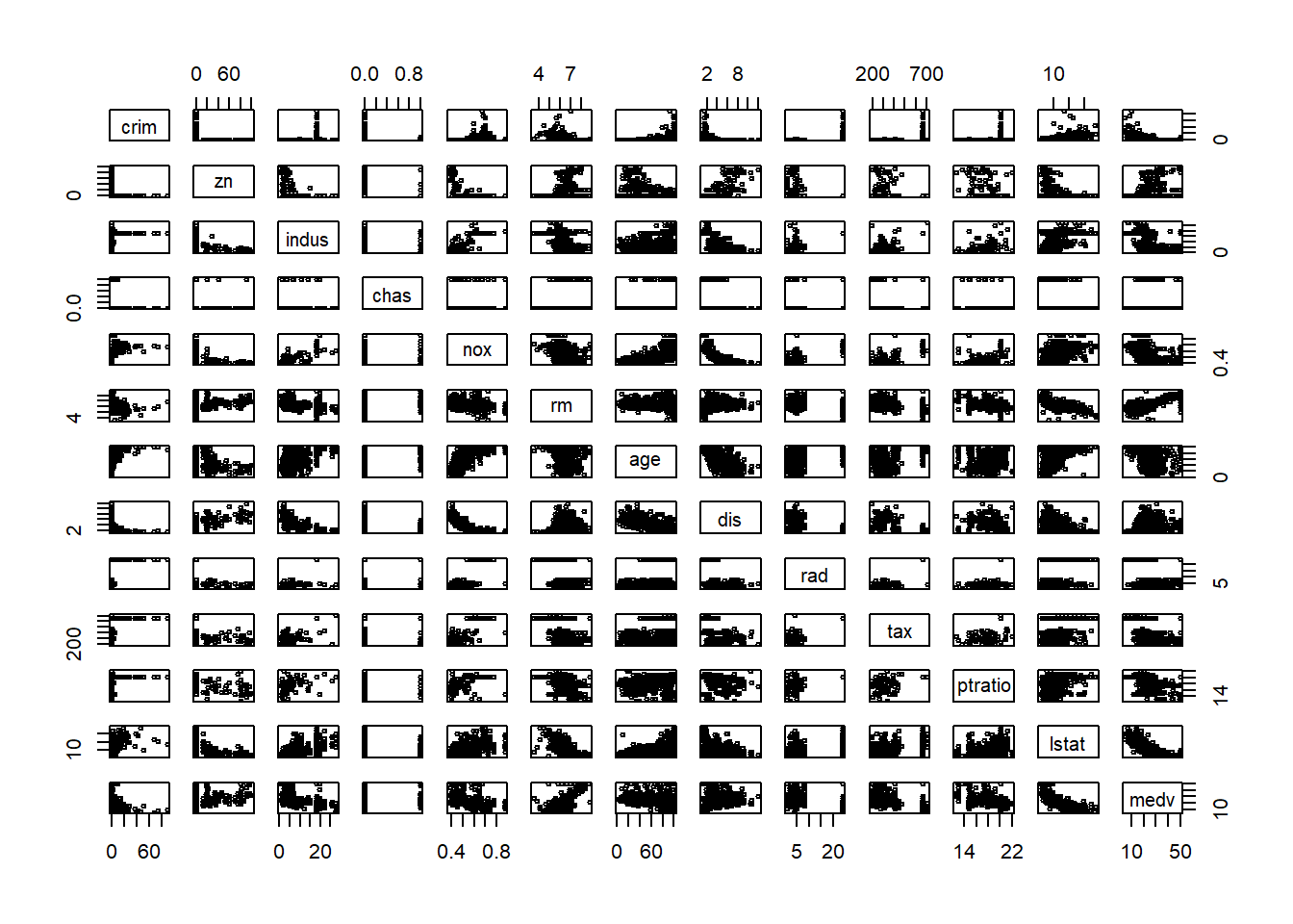
medv parameter has good positive correlation with rm and high negative correlation with lstat
indus parameter has high positive correlation with nox and tax, and high negative correlation with dis
and many more…

(c)

crm (per capita crime rate by town) has the highest correlation with rad (index of accesssibility to radial highways) which is positive.

(d)

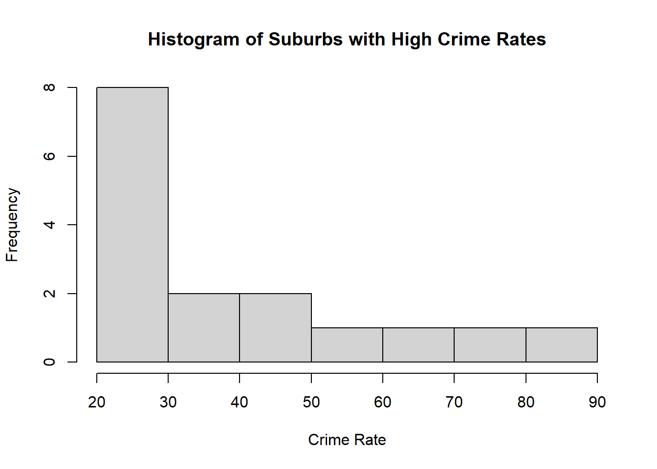
# High Crime Rates
High.Crime.Rate <- 
  Boston$crim[Boston$crim > mean(Boston$crim) + 2*sd(Boston$crim)]
cat("There are",length(High.Crime.Rate),"suburbs which have high crime rate")

There are 16 suburbs which have high crime rate

hist(High.Crime.Rate,
     xlab = "Crime Rate",
     main = "Histogram of Suburbs with High Crime Rates")

range(High.Crime.Rate)

[1] 22.0511 88.9762

# High Tax Rates
High.Tax.Rate <- 
  Boston$tax[Boston$tax > mean(Boston$tax) + 2*sd(Boston$tax)]

cat("There are",length(High.Tax.Rate), "suburbs which have high tax rate")

There are 0 suburbs which have high tax rate

# High Pupil-teacher ratios
High.Pupil.teacher.ratios <- 
  Boston$ptratio[Boston$ptratio > mean(Boston$ptratio) + 2*sd(Boston$ptratio)]

cat("There are",length(High.Pupil.teacher.ratios),
    "suburbs which have high Pupil-teacher ratio")

There are 0 suburbs which have high Pupil-teacher ratio

(e)

cat(“There are”,sum(Boston$chas),“suburbs that bound the Charles river.”)

(f)

cat(“Median pupil-teacher ratio in town is”,median(Boston$ptratio))

(g)

which(Boston$medv == min(Boston$medv))

[1] 399 406

# 399th and 406th

(h)

sum(Boston$rm > 7)

[1] 64

sum(Boston$rm > 8)

[1] 13

High.dwelling.Boston <- Boston[Boston$rm > 8, ]

summary(Boston)

      crim                zn             indus            chas        
 Min.   : 0.00632   Min.   :  0.00   Min.   : 0.46   Min.   :0.00000  
 1st Qu.: 0.08205   1st Qu.:  0.00   1st Qu.: 5.19   1st Qu.:0.00000  
 Median : 0.25651   Median :  0.00   Median : 9.69   Median :0.00000  
 Mean   : 3.61352   Mean   : 11.36   Mean   :11.14   Mean   :0.06917  
 3rd Qu.: 3.67708   3rd Qu.: 12.50   3rd Qu.:18.10   3rd Qu.:0.00000  
 Max.   :88.97620   Max.   :100.00   Max.   :27.74   Max.   :1.00000  
      nox               rm             age              dis        
 Min.   :0.3850   Min.   :3.561   Min.   :  2.90   Min.   : 1.130  
 1st Qu.:0.4490   1st Qu.:5.886   1st Qu.: 45.02   1st Qu.: 2.100  
 Median :0.5380   Median :6.208   Median : 77.50   Median : 3.207  
 Mean   :0.5547   Mean   :6.285   Mean   : 68.57   Mean   : 3.795  
 3rd Qu.:0.6240   3rd Qu.:6.623   3rd Qu.: 94.08   3rd Qu.: 5.188  
 Max.   :0.8710   Max.   :8.780   Max.   :100.00   Max.   :12.127  
      rad              tax           ptratio          lstat      
 Min.   : 1.000   Min.   :187.0   Min.   :12.60   Min.   : 1.73  
 1st Qu.: 4.000   1st Qu.:279.0   1st Qu.:17.40   1st Qu.: 6.95  
 Median : 5.000   Median :330.0   Median :19.05   Median :11.36  
 Mean   : 9.549   Mean   :408.2   Mean   :18.46   Mean   :12.65  
 3rd Qu.:24.000   3rd Qu.:666.0   3rd Qu.:20.20   3rd Qu.:16.95  
 Max.   :24.000   Max.   :711.0   Max.   :22.00   Max.   :37.97  
      medv      
 Min.   : 5.00  
 1st Qu.:17.02  
 Median :21.20  
 Mean   :22.53  
 3rd Qu.:25.00  
 Max.   :50.00

summary(High.dwelling.Boston)

      crim               zn            indus             chas       
 Min.   :0.02009   Min.   : 0.00   Min.   : 2.680   Min.   :0.0000  
 1st Qu.:0.33147   1st Qu.: 0.00   1st Qu.: 3.970   1st Qu.:0.0000  
 Median :0.52014   Median : 0.00   Median : 6.200   Median :0.0000  
 Mean   :0.71880   Mean   :13.62   Mean   : 7.078   Mean   :0.1538  
 3rd Qu.:0.57834   3rd Qu.:20.00   3rd Qu.: 6.200   3rd Qu.:0.0000  
 Max.   :3.47428   Max.   :95.00   Max.   :19.580   Max.   :1.0000  
      nox               rm             age             dis       
 Min.   :0.4161   Min.   :8.034   Min.   : 8.40   Min.   :1.801  
 1st Qu.:0.5040   1st Qu.:8.247   1st Qu.:70.40   1st Qu.:2.288  
 Median :0.5070   Median :8.297   Median :78.30   Median :2.894  
 Mean   :0.5392   Mean   :8.349   Mean   :71.54   Mean   :3.430  
 3rd Qu.:0.6050   3rd Qu.:8.398   3rd Qu.:86.50   3rd Qu.:3.652  
 Max.   :0.7180   Max.   :8.780   Max.   :93.90   Max.   :8.907  
      rad              tax           ptratio          lstat           medv     
 Min.   : 2.000   Min.   :224.0   Min.   :13.00   Min.   :2.47   Min.   :21.9  
 1st Qu.: 5.000   1st Qu.:264.0   1st Qu.:14.70   1st Qu.:3.32   1st Qu.:41.7  
 Median : 7.000   Median :307.0   Median :17.40   Median :4.14   Median :48.3  
 Mean   : 7.462   Mean   :325.1   Mean   :16.36   Mean   :4.31   Mean   :44.2  
 3rd Qu.: 8.000   3rd Qu.:307.0   3rd Qu.:17.40   3rd Qu.:5.12   3rd Qu.:50.0  
 Max.   :24.000   Max.   :666.0   Max.   :20.20   Max.   :7.44   Max.   :50.0

More average number of room per dwelling results in a lower crime rate